by Frederik Thomsen
Ordinary differential equations play a central part in mathematical modeling. They describe the change of quantities over time.
In the context of the EvoGamesPlus project, these quantities might represent the number of infected vs. healthy people in a pandemic, the number of various cancer cell types in a patient or the frequency with which certain strategies are played in a game, to name a few examples. The behavior of these models can be very complex. Famously, many differential equations display chaotic behavior, making it impossible to accurately predict the long-term behavior from an initial measurement of the quantities.
However, when a system can be modeled using only two quantities, the complexity is severely limited. This is often stated as “there is no chaos in two dimensions”. Formally, it is a consequence of the Poincaré-Bendixson theorem. The theorem states that the long-time behavior is limited to only three possibilities.
Subject of this blog post is gaining an idea of where these come from. This can be accomplished without any equations by simply drawing a few curves on a piece of paper (you are welcome to follow along).
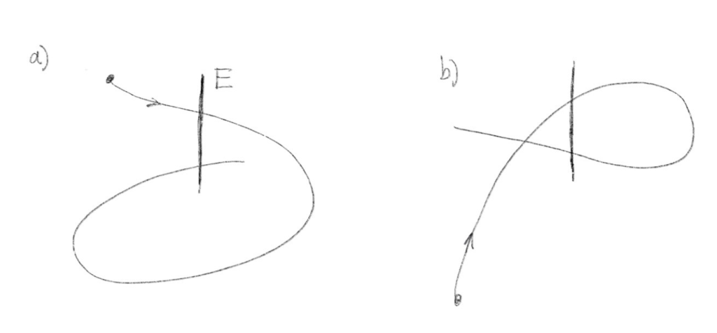
Let’s begin by drawing a line somewhere on the paper and call this line E. Now, choosing a starting point, we draw from it a single curve according to a set of rules:
- The curve must be drawn without lifting the pen off the paper
- The curve cannot cross over itself
- If the curve crosses through the line E, it must always do so in the same direction (for example left-to-right in sketch a).
To begin, we want to draw a curve that is closed, meaning we eventually loop back to our starting point. We find that such a curve cannot cross the line E more than once (see example c). Attempting to intersect it multiple times makes it impossible to close the curve without breaking the rules.
Next, we want to draw a curve that crosses through E three times. Let’s call the first intersection P1 and the second P2. As we continue drawing to add the third intersection P3, we find that it cannot lie between P1 and P2 (see example d).
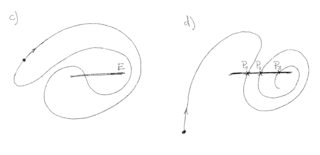
Next, we want to include curves drawn from different starting points and consider the long-term behavior. To this end, we add a fourth rule:
4. Curves drawn from different starting points cannot intersect.
Choosing our first starting point, let’s again draw a closed loop that intersects E in a point Q. The loop separates our canvas into two regions: one region “inside” and the other “outside” the loop. By rule 4, a curve started from either region will remain confined there. Let’s choose our second starting point “inside”, sharpen our pencil and draw a curve intersecting E many times. From our previous observation, as we add more and more intersections P1,P2,P3,P4,… we find them to be “ordered” along E always in the same direction, climbing toward Q or away from it. The resulting curve is forced to spiral in some way inward or outward (see example e). The situation is similar when starting in the “outside” region (example f).
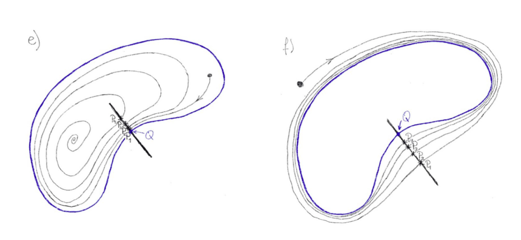
In the context of a differential equation, our starting point corresponds to the initial data. The piece of paper represents all possible values of the quantities. The curve (called “trajectory”) represents the changing values of the quantities over time, as determined by the model. The Poincaré-Bendixson theorem states the long term behavior of a trajectory must either include an equilibrium point (a point where the quantities no longer change over time) or a periodic orbit (a cycle in which points periodically repeat). In our drawing, an equilibrium point might be the end result of an inward spiral as depicted in example e). A periodic orbit is represented by a closed curve as depicted in f). In particular, if we have some means of knowing the trajectory cannot evolve toward an equilibrium, there must exist a periodic orbit in the system. With this periodic orbit we can associate again our E, Q and a sequence of intersections. If the sequence moves towards Q, accumulating more and more, we call the periodic orbit attracting.
In three or more dimensions, the situation is different. When we apply our set of rules, the observations made above are incorrect. A curve confined to some spatial volume for a very long time can fold in on itself in increasingly intricate ways. It is this folding that creates chaos.
Although the proof of Poincaré-Bendixson relies crucially on rules 2. and 4, similar limitations to complexity hold also for input-driven systems where these two rules do not apply. Examples of such systems are control systems. The control acts like an external force applied to the system, influencing the trajectory towards some specific goal. In the context of drawing curves, think of a someone else taking hold of your arm to steer. In the context of cancer therapy, the control might be the medication applied by the physician.
While the limitations make it significantly easier to predict the long-time behavior, it also severely restricts how much help the physician can actually provide to a patient.
If you are interested and want to learn more, keep an eye out for our upcoming preprint, where we leverage such limitations to identify global features in a minimal model for cancer therapy. For a detailed proof of the Poincaré-Bendixson theorem using the ideas above, check out for example Chapter 7 of Teschl “Ordinary differential equations and dynamical systems”. For related results in input-driven systems check out for example Chapter 3 of Filippov “Differential Equations with Discontinuous Righthand Sides”.

